B-splines in C2

Jon Maiga, 2020-06-29

After finishing a larger project I wanted to focus on something smaller and randomly picked up an old project where I used a b-spline setup to generate pretty smooth noise. For my own understanding, this post will go through the basics of b-splines and how to calculate certain coefficients.

B-splines use piecewise cubic polynomials that each interpolate between two consecutive points. To do this it requires additionally two neighboring points. We are only going to consider points with a constant space between them, or in the bigger picture, uniform b-splines.

I will denote the piecewise cubic curve that interpolates from $P_i$ to $P_{i+1}$ by $C_i(u)$ where $0\le u \le 1$. Note that I am using the term “interpolate” wrong since the curve is not necessarily passing through the control points.

What makes b-splines smooth is that we can get any wanted continuity, for C2 we have:

1. Positional continuity, interpolating will assure that neighbor points align $C_1(1)=C_2(0)$
2. Tangential continuity, interpolating will assure that the slopes of neighbor points align $C_1'(1)=C_2'(0)$
3. Curvature continuity, interpolating will assure that the curvature of neighbor points align $C_1''(1)=C_2''(0)$

To interpolate between the points $P_1$ and $P_2$ in C2 we additionally require the point to the left of $P_1$ and right of $P_2$, so we have to consider the four points $P_0,P_1,P_2,P_3$.

By using more control points and higher degree of the polynomials we can achieve any smoothness. For example, for C3 continuity requires fourth degree polynomials and five control points. This investigation will only consider C2.

The form of the cubic curve is $C_{1}(u)=a(u)P_0+b(u)P_1+c(u)P_2+d(u)P_3$ where $a(u), b(u), c(u), d(u)$ are weight functions for each control point those weight functions are called basis functions, which explains the name b(asis)-splines.

Basis functions

Each basis function takes a $0\le u \le1$ and outputs the weight of the corresponding point. The general form of our cubic basis function is

$B(u)=k_3u^3 + k_2u^2+ k_1u + k_0$

Here we will focus on one piecewise function, $C_1$. Since we have four control points, $P_0, P_1, P_2, P_3$ we get four corresponding basis functions

$a(u)=a_3u^3 + a_2u^2+ a_1u + a_0$
$b(u)=b_3u^3 + b_2u^2+ b_1u + b_0$
$c(u)=c_3u^3 + c_2u^2+ c_1u + c_0$
$d(u)=d_3u^3 + d_2u^2+ d_1u + d_0$

Each basis function will output the weight between $0$ and $1$, multiplying this with the corresponding point and summing all those gives us our cubic curve between the points $P_1$ and $P_2$.

$C_{1}(u)=a(u)P_0+b(u)P_1+c(u)P_2+d(u)P_3$

Deriving the basis coefficients

Now we need to figure out what the 16 coefficients are ($a_0-a_3, ..., d_0-d_3$). We have 16 unknown coefficients, so we will try to setup and solve a system of 16 equations in this step.

We already stated three constraints for the C2 guarantee,
$C_1(1)=C_2(0)$
$C_1'(1)=C_2'(0)$
$C_1''(1)=C_2''(0)$

Expanding the first of the three constraints we get
$a(1)P_0+b(1)P_1+c(1)P_2+d(1)P_3 + 0\cdot P_4 = 0\cdot P_0 + a(0)P_1+b(0)P_2+c(0)P_3+d(0)P_4$

We can write this as
$a(1)P_0 = 0\cdot P_0$
$b(1)P_1 = a(0)\cdot P_1$
$c(1)P_2 = b(0)\cdot P_2$
$d(1)P_3 = c(0)\cdot P_3$
$0\cdot P_4 = d(0)\cdot P_4$

Now we cancel the points and expands each basis function:

$\begin{cases} a_3+a_2+a_1+a_0=0 \\ b_3+b_2+b_1+b_0=a_0 \\ c_3+c_2+c_1+c_0=b_0 \\ d_3+d_2+d_1+d_0=c_0 \\ 0=d_0 \\ \end{cases}$

We end up with 5 equations, so 11 to go! We repeat the exact same procedure for the first and second derivatives and we get 10 additional equations. First we take the derivatives, e.g. for $a(u)$ we get:
$a'(u)=3a_3u^2+ 2a_2u +a_1$
$a''(u)=6a_3u+ 2a_2$

Then take the same steps as for before and from the first derivatives we end up with
$\begin{cases} 3a_3+2a_2+a_1=0 \\ 3b_3+2b_2+b_1=a_1 \\ 3c_3+2c_2+c_1=b_1 \\ 3d_3+2d_2+d_1=c_1 \\ 0=d_1 \end{cases}$

And from the second derivatives
$\begin{cases} 6a_3+2a_2=0 \\ 6b_3+2b_2=2a_2 \\ 6c_3+2c_2=2b_2 \\ 6d_3+2d_2=2c_2 \\ 0=2d_2 \\ \end{cases}$

Now we have 15 equations, but 16 unknowns so we need to add another. For the last one, we will add a new constraints that will keep our cubic in check, namely the sum of the weights of the of the basis functions should always equal to one, $a(u)+b(u)+c(u)+d(u)=1$. To achieve this we can consider the case when $u=0$, then we are only left with $a_0+b_0+c_0+d_0$ so clearly this has to add up to $1$.

$\begin{cases} a_0+b_0+c_0+d_0=1 \end{cases}$

After adding this last equation we can finally solve the equation system and retrive the coefficients. I was lazy and put it into Mathematica and got the following back

$[a_3, \dots, a_0] = \frac{1}{6}[-1,3,-3,1]$
$[b_3, \dots, b_0] = \frac{1}{6}[3,-6,0,4]$
$[c_3, \dots, c_0] = \frac{1}{6}[-3,3,3,1]$
$[d_3, \dots, d_0] = \frac{1}{6}[1,0,0,0]$

So we end up with the following set of cubics
$a(u)=\frac{1}{6}(-u^3+3u^2-3u+1)=\frac{1}{6}(1-u)^3$
$b(u)=\frac{1}{6}(3u^3-6u^2+4)$
$c(u)=\frac{1}{6}(-3u^3+3u^2+3u+1)$
$d(u)=\frac{1}{6}(u^3)$

and finally plugging this into $C$ gives us

$C_i(u)=\frac{1}{6}((1-u)^3P_{i-1}+(3u^3-6u^2+4)P_i+(-3u^3+3u^2+3u+1)P_{i+1}+u^3P_{i+2})$

Result

Plotting the individual basis functions in mathematica, you can see how the individual basis functions seamlessly goes from one another, $a(0)=b(1)$, $b(0)=c(1)$, $c(0)=d(1)$ and $d(0)=a(1)$. One can also guess that the sum of all four functions at any $u$ is $1$, just like our constraint wanted.

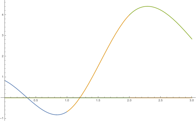
Here I am plotting three piecewise curves, to verify that it behaves as expected.

What is next?

The idea is to use b-splines to smoothen noise and see how it holds up against more common methods such as Perlin and Simplex noise. I decided to split each part into different posts and bring it all together in the last.

I used Uniform Cubic B-Spline Curves as a reference, it’s gives a really friendly walk-through!

Written with StackEdit.